3 Getting Started with R & RStudio
“Programming is like kicking yourself in the face, sooner or later your nose will bleed.” - Kyle Woodbury
A computer language is described by its syntax and semantics; where syntax is about the grammar of the language and semantics the meaning behind the sentence. And jumping into a new programming language correlates to visiting a foreign country with only that 9th grade Spanish 101 class under your belt; there is no better way to learn than to immerse yourself in the environment! Although it’ll be painful early on and your nose will surely bleed, eventually you’ll learn the dialect and the quirks that come along with it.
Throughout this book you’ll learn much of the fundamental syntax and semantics of the R programming language; and hopefully with minimal face kicking involved. However, this chapter serves to introduce you to many of the basics of R to get you comfortable. This includes installing R and RStudio, understanding the console, how to get help, how to work with packages, understanding how to assign and evaluate expressions, and the idea of vectorization. Finally, I offer some basic styling guidelines to help you write code that is easier to digest by others.
3.1 Installing R and RStudio
First, you need to download and install R, a free software environment for statistical computing and graphics from CRAN, the Comprehensive R Archive Network. It is highly recommended to install a precompiled binary distribution for your operating system; follow these instructions:
- Go to https://cran.r-project.org/
- Click “Download R for Mac/Windows”
- Download the appropriate file:
- Windows users click Base, and download the installer for the latest R version
- Mac users select the file R-4.X.X.pkg that aligns with your OS version
- Follow the instructions of the installer
Next, you can download RStudio’s IDE (integrated development environment), a powerful user interface for R. RStudio includes a text editor, so you do not have to install another stand-alone editor. Follow these instructions:
- Go to RStudio for desktop https://www.rstudio.com/products/rstudio/download/
- Select the install file for your OS
- Follow the instructions of the installer.
There are other R IDE’s available: Emacs, Microsoft R Open, Notepad++, etc; however, I have found RStudio to be my preferred route. When you are done installing RStudio click on the icon that looks like:
Figure 3.1: RStudio icon
and you should get a window that looks like the following:
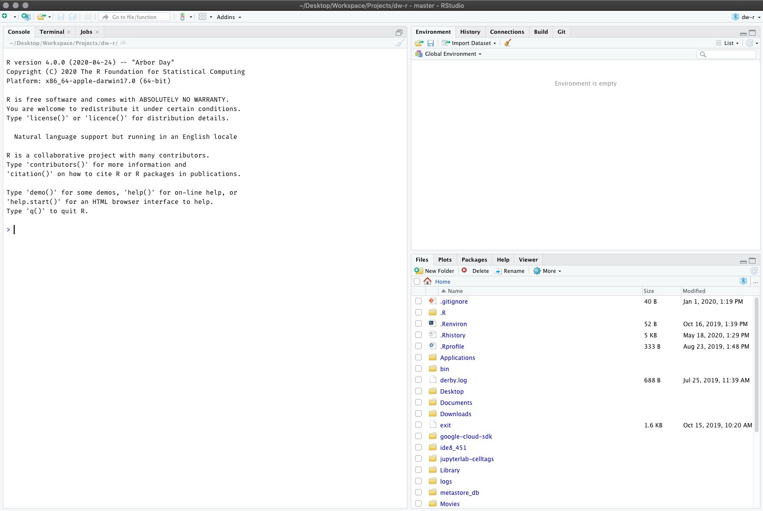
Figure 3.2: RStudio console
You are now ready to start programming!
3.2 Understanding the Console
The RStudio console is where all the action happens. There are four fundamental windows in the console, each with their own purpose. I discuss each briefly below but I highly suggest Oscar Torres-Reyna’s Introduction to RStudio for a thorough understanding of the console7.
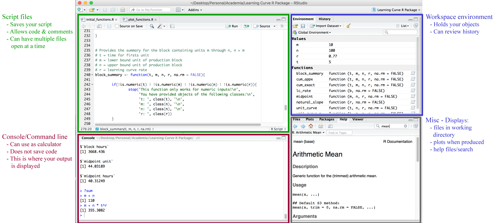
Figure 3.3: The four fundamental windows within the RStudio IDE
3.2.1 Script Editor
The top left window is where your script files will display. There are multiple forms of script files but the basic one to start with is the .R file. To create a new file you use the File » New File menu. To open an existing file you use either the File » Open File… menu or the Recent Files menu to select from recently opened files. RStudio’s source editor includes a variety of productivity enhancing features including syntax highlighting, code completion, multiple-file editing, and find/replace. A good introduction to the script editor was written by RStudio’s Josh Paulson8.
The script editor is a great place to put code you care about. Keep experimenting in the console, but once you have written code that works and does what you want, put it in the script editor. RStudio will automatically save the contents of the editor when you quit RStudio, and will automatically load it when you re-open. Nevertheless, it’s a good idea to save your scripts regularly and to back them up.
To execute the code in the script editor you have two options:
- Place the cursor on the line that you would like to execute and execute Cmd/Ctrl + Enter. Alternatively, you could hit the Run button in the toolbar.
- If you want to run all lines of code in the script then you can highlight the lines you want to run and then execute one of the options in #1.
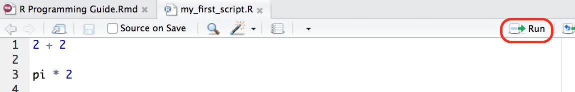
Figure 3.4: Execute lines of code in your script with Cmd/Ctrl + Enter or using the Run button.
3.2.2 Workspace Environment
The top right window is the workspace environment which captures much of your your current R working environment and includes any user-defined objects (vectors, matrices, data frames, lists, functions). When saving your R working session, these are the components along with the script files that will be saved in your working directory, which is the default location for all file inputs and outputs. To get or set your working directory so you can direct where your files are saved:
# returns path for the current working directory
getwd()

# set the working directory to a specified directory
setwd("path/of/directory")
For example, if I call getwd() the file path “/Users/b294776/Desktop/Workspace/Projects/dw-r” is returned. If I want to set the working directory to the “Workspace” folder within the “Desktop” directory I would use setwd("/Users/b294776/Desktop/Workspace"). Now if I call getwd() again it returns “/Users/b294776/Desktop/Workspace”. An alternative solution is to go to the following location in your toolbar Session » Set Working Directory » Choose Directory and select the directory of choice (much easier!).
The workspace environment will also list your user defined objects such as vectors, matrices, data frames, lists, and functions. For example, if you type the following in your console:
You will now see x and y listed in your workspace environment. To identify or remove the objects (i.e. vectors, data frames, user defined functions, etc.) in your current R environment:
# list all objects
ls()

# identify if an R object with a given name is present
exists("x")

# remove defined object from the environment
rm(x)

# you can remove multiple objects
rm(x, y)

# basically removes everything in the working environment -- use with caution!
rm(list = ls())
If you have a lot of objects in your workspace environment you can use the 🧹 icon in the workspace environment tab to clear out everything.
You can also view previous commands in the workspace environment by clicking the History tab, by simply pressing the up arrow on your keyboard, or by typing into the console:
3.2.3 Console
The bottom left window contains the console. You can code directly in this window but it will not save your code. It is best to use this window when you are simply wanting to perform calculator type functions. This is also where your outputs will be presented when you run code in your script. Go ahead and type the following in your console:
3.2.4 Misc. Displays
The bottom right window contains multiple tabs. The Files tab allows you to see which files are available in your working directory. The Plots tab will display any plots/graphics that are produced by your code. The Packages tab will list all packages downloaded to your computer and also the ones that are loaded (more on this later). And the Help tab allows you to search for topics you need help on and will also display any help responses (more on this later as well).
3.2.5 Workspace Options & Shortcuts
There are multiple options available for you to set and customize both R and your RStudio console. For R, you can read about, and set, available options for the current R session with the following code. For now you don’t need to worry about making any adjustments, just know that many options do exist.
# learn about available options
help(options)

# view current option settings
options()

# change a specific option (i.e. number of digits to print on output)
options(digits=3)
For a thorough tutorial regarding the RStudio console and how to customize different components check out this tutorial. You can also find the RStudio console cheatsheet shown below here or by going to Help menu » Cheatsheets. As with most computer programs, there are numerous keyboard shortcuts for working with the console. To access a menu displaying all the shortcuts in RStudio you can use option + shift + k. Within RStudio you can also access them in the Help menu » Keyboard Shortcuts.
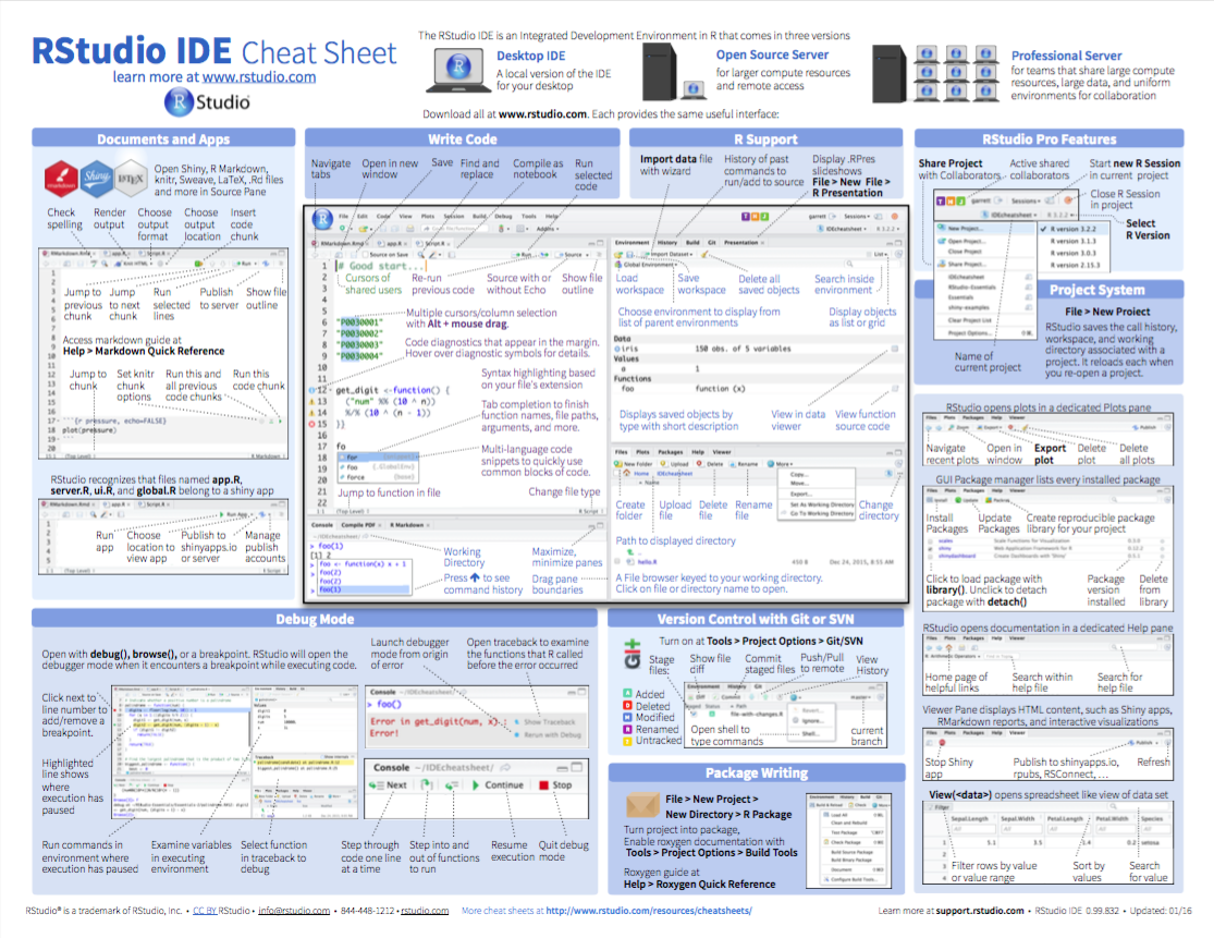
Figure 3.5: RStudio IDE cheat sheet.
3.2.6 Exercises
- Identify what working directory you are working out of.
- Create a folder on your computer titled Learning R. Within R, set your working directory to this folder.
- Type
piin the console. Set the option to show 8 digits. Re-typepiin the console. - Type
?piin the console. Note that documentation on this object pops up in the Help tab in the Misc. Display. - Now check out your code History tab.
- Create a new .R file and save this as my-first-script (note how this now appears in your Learning R folder). Type
piin line 1 of this script,option(digits = 8)in line 2, andpiagain in line three. Execute this code one line at a time and then re-execute all lines at once.
3.3 Getting Help
The help documentation and support in R is comprehensive and easily accessible from the the console.
3.3.1 General Help
To leverage general help resources you can use:
# provides general help links
help.start()

# searches the help system for documentation matching a given character string
help.search("linear regression")
Note that the help.search("some text here") function requires a character string enclosed in quotation marks. So if you are in search of time series functions in R, using help.search("time series") will pull up a healthy list of vignettes and code demonstrations that illustrate packages and functions that work with time series data.
3.3.2 Getting Help on Functions
For more direct help on functions that are installed on your computer you can use the following. Test these out in your console:
help(mean)      # provides details for specific function
?mean           # provides same information as help(functionname)
example(mean)   # provides examples for said function
Note that the help() and ? function calls only work for functions within loaded packages. You’ll understand what this means shortly.
3.3.3 Getting Help From the Web
Typically, a problem you may be encountering is not new and others have faced, solved, and documented the same issue online. The following resources can be used to search for online help. Although, I typically just Google the problem and find answers relatively quickly.
RSiteSearch("key phrase"): searches for the key phrase in help manuals and archived mailing lists on the R Project website.- Stack Overflow: a searchable Q&A site oriented toward programming issues. 75% of my answers typically come from Stack Overflow.
- Cross Validated: a searchable Q&A site oriented toward statistical analysis.
- RStudio Community: a community for all things R and RStudio where you can get direct answers to your problems and also give back by helping to solve and answer other’s questions.
- R-seek: a Google custom search that is focused on R-specific websites
- R-bloggers: a central hub of content collected from over 500 bloggers who provide news and tutorials about R.
Although Twitter has a thriving R community, it is not the place to ask for help on specific code functionality.
3.4 Working with Packages
In R, the fundamental unit of share-able code is the package. A package bundles together code, data, documentation, and tests and provides an easy method to share with others (Wickham 2015). As of May 2020 there were over 15,000 packages available on CRAN, 1900 on Bioconductor, and countless more available through GitHub. This huge variety of packages is one of the reasons that R is so successful: chances are that someone has already solved a problem that you’re working on, and you can benefit from their work by downloading their package.
3.4.1 Installing Packages
The most common place to get packages from is CRAN. To install packages from CRAN you use install.packages("packagename"). For instance, if you want to install the ggplot2 package, which is a very popular visualization package you would type the following in the console:
As previously stated, packages are also available through Bioconductor and GitHub. Bioconductor provides R packages primarily for genomic data analyses and packages on GitHub are usually under development but have not gone through all the checks and balances to be loaded onto CRAN (aka download and use these packages at your discretion). You can learn how to install Bioconductor packages here and GitHub packages here.
3.4.2 Loading Packages
Once the package is downloaded to your computer you can access the functions and resources provided by the package in two different ways:
# load the package to use in the current R session
library(packagename)

# use a particular function within a package without loading the package
packagename::functionname
For instance, if you want to have full access to the tidyr package you would use library(tidyr); however, if you just wanted to use the gather() function which is provided by the tidyr package without fully loading tidyr you can use tidyr::gather(...)9.
3.4.3 Getting Help on Packages
For more direct help on packages that are installed on your computer you can use the help and vignette functions. Here we can get help on the ggplot2 package with the following:
help(package = "ggplot2")      # provides details regarding contents of a package
vignette(package = "ggplot2")  # list vignettes available for a specific package
vignette("ggplot2-specs")      # view specific vignette
vignette()                     # view all vignettes on your computer
Note that some packages will have multiple vignettes. For instance vignette(package = "grid") will list the 13 vignettes available for the grid package. To access one of the specific vignettes you simply use vignette("vignettename").
3.4.4 Useful Packages
There are thousands of helpful R packages for you to use, but navigating them all can be a challenge. To help you out, RStudio compiled a guide to some of the best packages for loading, manipulating, visualizing, analyzing, and reporting data. In addition, their list captures packages that specialize in spatial data, time series and financial data, increasing spead and performance, and developing your own R packages.
3.4.5 Exercises
dplyr is an extremely popular package for common data transformation activities and is available from CRAN. Perform the following tasks:
- Install the dplyr package.
- Load the dplyr package.
- Access the help documentation for the dplyr package.
- Check out the vignette(s) for dplyr.
3.5 Assignment & Evaluation
3.5.1 Assignment
The first operator you’ll run into is the assignment operator. The assignment operator is used to assign a value. For instance we can assign the value 3 to the variable x using the <- assignment operator.
R is a dynamically typed programming language which means it will perform the process of verifying and enforcing the constraints of types at run-time. If you are unfamiliar with dynamically versus statically-typed languages then do not worry about this detail. Just realize that dynamically typed languages allow for the simplicity of running the above command and R automatically inferring that 3 should be a numeric type rather than a character string.
Interestingly, R actually allows for five assignment operators10:
# leftward assignment
x <- value
x = value
x <<- value

# rightward assignment
value -> x
value ->> x
The original assignment operator in R was <- and has continued to be the preferred among R users. The = assignment operator was added in 2001 primarily because it is the accepted assignment operator in many other languages and beginners to R coming from other languages were so prone to use it. Using = is not wrong, just realize that most R programmers prefer to keep = reserved for argument association and use <- for assignment.
The operators <<- is normally only used in functions or looping constructs which we will not get into the details. And the rightward assignment operators perform the same as their leftward counterparts, they just assign the value in an opposite direction.
Overwhelmed yet? Don’t be. This is just meant to show you that there are options and you will likely come across them sooner or later. My suggestion is to stick with the tried, true, and idiomatic <- operator. This is the most conventional assignment operator used and is what you will find in all the base R source code…which means it should be good enough for you.
3.5.2 Evaluation
We can then evaluate the variable by simply typing x at the command line which will return the value of x. Note that prior to the value returned you’ll see ## [1] in the console. This simply implies that the output returned is the first output. Note that you can type any comments in your code by preceding the comment with the hash tag (#) symbol. Any values, symbols, and texts following # will not be evaluated.
3.5.3 Case Sensitivity
Lastly, note that R is a case sensitive programming language. Meaning all variables, functions, and objects must be called by their exact spelling:
3.5.4 Exercises
- Assign the value 5 to variable
x(note how this shows up in your Global Environment). - Assign the character
“abc”to variabley. - Evaluate the value of
xandyat in the console. - Now use the
rm()function to remove these objects from you working environment.
3.6 R as a Calculator
3.6.1 Basic Arithmetic
At its most basic function R can be used as a calculator. When applying basic arithmetic, the PEMDAS order of operations applies: parentheses first followed by exponentiation, multiplication and division, and finally addition and subtraction.
8 + 9 / 5 ^ 2
## [1] 8.36

8 + 9 / (5 ^ 2)
## [1] 8.36

8 + (9 / 5) ^ 2
## [1] 11.24

(8 + 9) / 5 ^ 2
## [1] 0.68
By default R will display seven digits but this can be changed using options() as previously outlined.
Also, large numbers will be expressed in scientific notation which can also be adjusted using options().
Note that the largest number of digits that can be displayed is 22. Requesting any larger number of digits will result in an error message.
pi
## [1] 3.141592654

options(digits = 22)
pi
## [1] 3.141592653589793115998

options(digits = 23)
## Error in options(digits = 23): invalid 'digits' parameter, allowed 0...22
pi
## [1] 3.141592653589793115998
We can also perform integer divide (%/%) and modulo (%%) functions. The integer divide function will give the integer part of a fraction while the modulo will provide the remainder.
3.6.2 Miscellaneous Mathematical Functions
There are many built-in functions to be aware of. These include but are not limited to the following. Go ahead and run this code in your console.
3.6.3 Infinite, and NaN Numbers
When performing undefined calculations, R will produce Inf (infinity) and NaN (not a number) outputs. These can easily pop up in regular data wrangling tasks and later chapters will discuss how to work with these types of outputs along with missing values.
3.6.4 Exercises
- Assign the values 1000, 5, and 0.05 to variables
D,K, andhrespectively. - Compute \(2 \times D \times K\).
- Compute \(\frac{2 \times D \times K}{h}\).
- Now put this together to compute the Economic Order Quantity, which is \(\sqrt{\frac{2 \times D \times K}{h}}\). Save the output as
Q.
3.7 Vectorization
3.7.1 Looping versus Vectorization
A key difference between R and many other languages is a topic known as vectorization. What does this mean? It means that many functions that are to be applied individually to each element in a vector of numbers require a loop assessment to evaluate; however, in R many of these functions have been coded in C to perform much faster than a for loop would perform. For example, let’s say you want to add the elements of two separate vectors of numbers (x and y).
In other languages you might have to run a loop to add two vectors together. In this for loop I print each iteration to show that the loop calculates the sum for the first elements in each vector, then performs the sum for the second elements, etc.
# empty vector to store results
z <- as.vector(NULL)

# `for` loop to add corresponding elements in each vector
for (i in seq_along(x)) {
        z[i] <- x[i] + y[i]
        print(z)
}
## [1] 2
## [1] 2 5
## [1] 2 5 8
Instead, in R, + is a vectorized function which can operate on entire vectors at once. So rather than creating for loops for many functions, you can just use simple syntax:
3.7.2 Recycling
When performing vector operations in R, it is important to know about recycling. When performing an operation on two or more vectors of unequal length, R will recycle elements of the shorter vector(s) to match the longest vector. For example:
long <- 1:10
short <- 1:5

long
##  [1]  1  2  3  4  5  6  7  8  9 10
short
## [1] 1 2 3 4 5

long + short
##  [1]  2  4  6  8 10  7  9 11 13 15
The elements of long and short are added together starting from the first element of both vectors. When R reaches the end of the short vector, it starts again at the first element of short and continues until it reaches the last element of the long vector. This functionality is very useful when you want to perform the same operation on every element of a vector. For example, say we want to multiply every element of our vector long by 3:
There are no scalars in R, so c is actually a vector of length 1; in order to add its value to every element of long, it is recycled to match the length of long.
Don’t get hung up with some of the verbiage used here (i.e. vectors, scalars), we will cover what this means in later chapters.
When the length of the longer object is a multiple of the shorter object length, the recycling occurs silently. When the longer object length is not a multiple of the shorter object length, a warning is given:
3.7.3 Exercises
- Create this vector
my_vec <- 1:10. - Add 1 to every element in
my_vec. - Divide every element in
my_vecby 2. - Create a second vector
my_vec2 <- 10:18and addmy_vectomy_vec2.
3.8 Style Guide
“Good coding style is like using correct punctuation. You can manage without it, but it sure makes things easier to read.” - Hadley Wickham
As a medium of communication, its important to realize that the readability of code does in fact make a difference. Well styled code has many benefits to include making it easy to i) read, ii) extend, and iii) debug. Unfortunately, R does not come with official guidelines for code styling but such is an inconvenient truth of most open source software. However, this should not lead you to believe there is no style to be followed and over time implicit guidelines for proper code styling have been documented.
What follows are a few of the basic guidelines from the tidyverse style guide. These suggestions will help you get started with good styling suggestions as you begin this book but as you progress you should leverage the far more detailed tidyverse style guide along with useful packages such as lintr and styler to help enforce good code syntax on yourself.
3.8.1 Notation and Naming
File names should be meaningful and end with a .R extension.
If files need to be run in sequence, prefix them with numbers:
In R, naming conventions for variables and functions are famously muddled. They include the following:
namingconvention        # all lower case; no separator
naming.convention       # period separator
naming_convention       # underscore separator (aka snake case)
namingConvention        # lower camel case
NamingConvention        # upper camel case
Historically, there has been no clearly preferred approach with multiple naming styles sometimes used within a single package. Bottom line, your naming convention will be driven by your preference but the ultimate goal should be consistency.
My personal preference is to use all lowercase with an underscore ("_") to separate words within a name. Furthermore, variable names should be nouns and function names should be verbs to help distinguish their purpose. Also, refrain from using existing names of functions (i.e. mean, sum, true).
3.8.2 Organization
Organization of your code is also important. There’s nothing like trying to decipher 500 lines of code that has no organization. The easiest way to achieve organization is to comment your code. When you have large sections within your script you should separate them to make it obvious of the distinct purpose of the code.
# Download Data -------------------------------------------------------------------
lines of code here

# Preprocess Data -----------------------------------------------------------------
lines of code here

# Exploratory Analysis ------------------------------------------------------------
lines of code here
You can easily add these section breaks within RStudio wth Cmd+Shift+R.
Then comments for specific lines of code can be done as follows:
code_1  # short comments can be placed to the right of code
code_2  # blah
code_3  # blah

# or comments can be placed above a line of code
code_4

# Or extremely long lines of commentary that go beyond the suggested 80
# characters per line can be broken up into multiple lines. Just don't forget
# to use the hash on each.
code_5
You can easily comment or uncomment lines by highlighting the line and then pressing Cmd+Shift+C.
3.8.3 Syntax
The maximum number of characters on a single line of code should be 80 or less. If you are using RStudio you can have a margin displayed so you know when you need to break to a new line11. Also, when indenting your code use two spaces rather than using tabs. The only exception is if a line break occurs inside parentheses. In this case it is common to do either of the following:
# option 1
super_long_name <- seq(ymd_hm("2015-1-1 0:00"),
                       ymd_hm("2015-1-1 12:00"),
                       by = "hour")

# option 2
super_long_name <- seq(
  ymd_hm("2015-1-1 0:00"),
  ymd_hm("2015-1-1 12:00"),
  by = "hour"
)
Proper spacing within your code also helps with readability. Place spaces around all infix operators (=, +, -, <-, etc.). The same rule applies when using = in function calls. Always put a space after a comma, and never before.
# Good
average <- mean(feet / 12 + inches, na.rm = TRUE)

# Bad
average<-mean(feet/12+inches,na.rm=TRUE)
There’s a small exception to this rule: :, :: and ::: don’t need spaces around them.
It is important to think about style when communicating any form of language. Writing code is no exception and is especially important if your code will be read by others. Following these basic style guides will get you on the right track for writing code that can be easily communicated to others.
3.8.4 Exercises
Go back through the script you’ve been writing to execute the exercises in this chapter and make sure
- your naming conventions are consistent,
- your code is nicely organized and annotated,
- your syntax includes proper spacing.
References
Wickham, Hadley. 2015. R Packages: Organize, Test, Document, and Share Your Code. " O’Reilly Media, Inc.".
You can access this tutorial at http://dss.princeton.edu/training/RStudio101.pdf. Note that although it is from 2013 it still is very applicable and does a very thorough introduction↩
You can assess the script editor tutorial at https://support.rstudio.com/hc/en-us/articles/200484448-Editing-and-Executing-Code↩
Here,
...just represents the arguments that you would include in this function↩There are even more provided by third party packages such as zeallot.↩
Tools » Global Options » Code » Display↩